Note
Go to the end to download the full example code.
Flare List Demo#
How to search, combine and explore STIX L3 flare list products.
This example uses STIXClient (a Fido client) to find
three months of L3 flare list files, loads each one as a
FlareList product, concatenates them
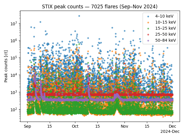
into a single catalogue, plots the peak count time series, then filters for
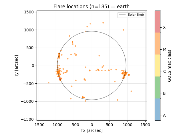
X-class flares close to the Earth-facing solar limb and plots their locations.
Imports
import matplotlib.pyplot as plt
import numpy as np

from sunpy.net import attrs as a

from stixpy.net.client import STIXClient
from stixpy.product import Product
Search three months of flare list data.
The flare list test products are currently hosted on a separate URL from the
rest of the STIX archive, so we instantiate STIXClient
with that source.
client = STIXClient(source="https://pub099.cs.technik.fhnw.ch/testing/p311_comp_test")

results = client.search(
    a.Time("2024-09-01T01:00:00", "2024-11-30T23:59"),
    a.Instrument.stix,
    a.stix.DataType.flarelist,
)
print(results)
       Start Time               End Time        Instrument Level  DataType   DataProduct    Ver Request ID
----------------------- ----------------------- ---------- ----- --------- ---------------- --- ----------
2024-09-01T00:00:00.000 2024-10-01T00:47:10.000       STIX    L3 FLARELIST flarelist-sdcloc V02          -
2024-10-01T00:00:00.000 2024-11-01T00:05:46.000       STIX    L3 FLARELIST flarelist-sdcloc V02          -
2024-11-01T00:00:00.000 2024-11-30T23:48:24.000       STIX    L3 FLARELIST flarelist-sdcloc V02          -
Download the matching files and load each one as a FlareList product
paths = client.fetch(results)
products = [Product(p) for p in paths]
Files Downloaded:   0%|          | 0/3 [00:00<?, ?file/s]


solo_L3_stix-flarelist-sdcloc_20241101T000000-20241130T234824_V02.fits:   0%|          | 0.00/1.22M [00:00<?, ?B/s]


solo_L3_stix-flarelist-sdcloc_20241001T000000-20241101T000546_V02.fits:   0%|          | 0.00/1.44M [00:00<?, ?B/s]

solo_L3_stix-flarelist-sdcloc_20240901T000000-20241001T004710_V02.fits:   0%|          | 0.00/1.35M [00:00<?, ?B/s]


solo_L3_stix-flarelist-sdcloc_20241001T000000-20241101T000546_V02.fits:   0%|          | 1.02k/1.44M [00:00<02:44, 8.72kB/s]


solo_L3_stix-flarelist-sdcloc_20241101T000000-20241130T234824_V02.fits:   0%|          | 1.02k/1.22M [00:00<02:22, 8.54kB/s]

solo_L3_stix-flarelist-sdcloc_20240901T000000-20241001T004710_V02.fits:   0%|          | 1.02k/1.35M [00:00<02:35, 8.70kB/s]


solo_L3_stix-flarelist-sdcloc_20241101T000000-20241130T234824_V02.fits:   1%|          | 8.94k/1.22M [00:00<00:26, 44.9kB/s]


solo_L3_stix-flarelist-sdcloc_20241001T000000-20241101T000546_V02.fits:   1%|          | 8.94k/1.44M [00:00<00:31, 44.9kB/s]

solo_L3_stix-flarelist-sdcloc_20240901T000000-20241001T004710_V02.fits:   1%|          | 8.94k/1.35M [00:00<00:30, 44.4kB/s]


solo_L3_stix-flarelist-sdcloc_20241101T000000-20241130T234824_V02.fits:   3%|▎         | 40.9k/1.22M [00:00<00:07, 160kB/s]


solo_L3_stix-flarelist-sdcloc_20241001T000000-20241101T000546_V02.fits:   3%|▎         | 40.9k/1.44M [00:00<00:08, 157kB/s]

solo_L3_stix-flarelist-sdcloc_20240901T000000-20241001T004710_V02.fits:   3%|▎         | 40.9k/1.35M [00:00<00:08, 160kB/s]


solo_L3_stix-flarelist-sdcloc_20241101T000000-20241130T234824_V02.fits:  11%|█         | 129k/1.22M [00:00<00:02, 420kB/s]


solo_L3_stix-flarelist-sdcloc_20241001T000000-20241101T000546_V02.fits:   9%|▉         | 129k/1.44M [00:00<00:03, 419kB/s]

solo_L3_stix-flarelist-sdcloc_20240901T000000-20241001T004710_V02.fits:  10%|▉         | 129k/1.35M [00:00<00:02, 420kB/s]


solo_L3_stix-flarelist-sdcloc_20241101T000000-20241130T234824_V02.fits:  26%|██▌       | 313k/1.22M [00:00<00:01, 885kB/s]


solo_L3_stix-flarelist-sdcloc_20241001T000000-20241101T000546_V02.fits:  23%|██▎       | 337k/1.44M [00:00<00:01, 962kB/s]

solo_L3_stix-flarelist-sdcloc_20240901T000000-20241001T004710_V02.fits:  25%|██▍       | 337k/1.35M [00:00<00:01, 963kB/s]


solo_L3_stix-flarelist-sdcloc_20241101T000000-20241130T234824_V02.fits:  52%|█████▏    | 629k/1.22M [00:00<00:00, 1.58MB/s]


solo_L3_stix-flarelist-sdcloc_20241001T000000-20241101T000546_V02.fits:  47%|████▋     | 672k/1.44M [00:00<00:00, 1.69MB/s]

solo_L3_stix-flarelist-sdcloc_20240901T000000-20241001T004710_V02.fits:  48%|████▊     | 655k/1.35M [00:00<00:00, 1.64MB/s]


solo_L3_stix-flarelist-sdcloc_20241101T000000-20241130T234824_V02.fits:  87%|████████▋ | 1.06M/1.22M [00:00<00:00, 2.37MB/s]


solo_L3_stix-flarelist-sdcloc_20241001T000000-20241101T000546_V02.fits:  77%|███████▋  | 1.11M/1.44M [00:00<00:00, 2.47MB/s]

solo_L3_stix-flarelist-sdcloc_20240901T000000-20241001T004710_V02.fits:  79%|███████▉  | 1.07M/1.35M [00:00<00:00, 2.36MB/s]


Files Downloaded:  33%|███▎      | 1/3 [00:01<00:02,  1.14s/file]


Files Downloaded: 100%|██████████| 3/3 [00:01<00:00,  2.61file/s]
Concatenate the monthly products into a single FlareList covering Sep–Nov 2024
flares = products[0].concatenate(products[1:])
print(flares)
FlareList
       <sunpy.time.timerange.TimeRange object at 0x7125fd895c40>
    Start: 2024-09-01 00:06:44
    End:   2024-11-30 23:48:24
    Center:2024-10-16 11:57:34
    Duration:90.98726238425925 days or
           2183.6942972222223 hours or
           131021.65783333333 minutes or
           7861299.47 seconds

    7025 flares
Inspect the available columns. flares.data is an
QTable — each column carries its own unit and a
short description loaded from the FITS header.
print(f"{'Column':<26s}  {'Unit':<10s}  Description")
print("-" * 90)
for name in flares.data.colnames:
    info = flares.data[name].info
    unit = "" if info.unit is None else str(info.unit)
    desc = info.description or ""
    print(f"{name:<26s}  {unit:<10s}  {desc}")
Column                      Unit        Description
------------------------------------------------------------------------------------------
flare_id                                unique flare id for flarelist SDCFlareListManager
start_UTC                               start time of flare
duration                    s           duration of flare
end_UTC                                 end time of flare
peak_UTC                                flare peak time
att_in                                  was attenuator in during flare
bkg_baseline                ct          background baseline at 4-10 keV
GOES_class                              GOES class of the GOES XRS data at time of flare - not derived from STIX data.  Do not use when flare isn't visible to Earth
goes_min_class_est                      min GOES class estimate derived from STIX data
goes_max_class_est                      max GOES class estimate derived from STIX data
goes_mean_class_est                     mean GOES class estimate derived from STIX data
GOES_flux                   W / m2      GOES flux of the GOES XRS data at time of flare- not derived from STIX data. Do not use when the flare isn't visible to Earth
goes_min_flux_est           W / m2      min GOES flux estimate derived from STIX data
goes_max_flux_est           W / m2      max GOES flux estimate derived from STIX data
goes_mean_flux_est          W / m2      mean GOES flux estimate derived from STIX data
lc_peak                     ct          counts in 4s peak window from quicklook lightcurve
lc_bgk_peak                 ct          background counts in 4s peak windowfrom quicklook lightcurve
energy_index                            energy band index
soop_encoded_type                       campaign ID
soop_id                                 SOOP ID
soop_type                               name of the SOOP campaign
anc_ephemeris_path                      Path to the daily ancillary ephemeris file
cpd_path                                Path to the CPD file used for flare location estimation
_position_status                        Status of the flare position calculation
_position_message                       Message describing the status of the flare position calculation
location_icrs               deg,deg,km  Flare location in ICRS coordinates at 'location_time_UTC'
solo_location_icrs          deg,deg,km  Solar Orbiter location in ICRS coordinates at 'location_time_UTC'
sidelobes_ratio                         Ratio of sidelobes in the STIX image used to assess imaging quality
rcr_at_peak                             max rcr level at flare location estimation time range, > 0 attenuator in place
visible_from_earth                      Whether the flare location is visible from Earth (not occulted by the Sun)
location_time_UTC                       time center used for flare location estimation in UTC
location_duration           s           duration of the flare location estimation time range
time_shift                  s           Time(Sun to Earth) - Time(Sun to S/C)
sun_disc_size               arcsec      Apparent photospheric solar radius
location_hgs                deg,deg,km  Flare location in Heliographic Stonyhurst coordinates at 'location_time_UTC'
solo_location_hgs           deg,deg,km  Solar Orbiter location in Heliographic Stonyhurst coordinates at 'location_time_UTC'
Plot the timeline of peak counts per energy band across all three months
flares.plot_timeseries()
plt.title(f"STIX peak counts — {len(flares)} flares (Sep–Nov 2024)")
plt.tight_layout()
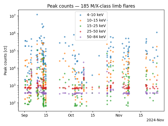
Filter the catalogue for M- and X-class flares close to the Earth-facing limb.
Seen from Earth the solar limb maps to HGS longitude ±90°. We keep flares
whose absolute HGS longitude exceeds 70° and whose GOES classification starts
with "M" or "X".
lon = flares.flare_location_hgs.lon.deg
is_strong = np.array([str(g).strip().upper().startswith(("M", "X")) for g in flares.goes_class])
near_limb = np.isfinite(lon) & (np.abs(lon) > 70)
mask = is_strong & near_limb
print(f"Selected {mask.sum()} M/X-class limb flares of {len(flares)} total.")
Selected 185 M/X-class limb flares of 7025 total.
A boolean mask can be applied directly to the FlareList; the result is a new FlareList with the matching rows. Plot the filtered locations from Earth’s point of view.
filtered = flares[mask]
print(filtered)

filtered.plot_timeseries()
plt.title(f"Peak counts — {len(filtered)} M/X-class limb flares")
plt.tight_layout()

filtered.plot_locations(observer="earth")
plt.tight_layout()
FlareList
       <sunpy.time.timerange.TimeRange object at 0x7125fd760f80>
    Start: 2024-09-01 07:56:24
    End:   2024-11-25 17:22:01
    Center:2024-10-14 00:39:13
    Duration:85.39278921296297 days or
           2049.4269411111113 hours or
           122965.61646666667 minutes or
           7377936.988 seconds

    185 flares
Masking is non-destructive: flares is the full catalogue, so we can
apply a completely independent filter to the same object — here, strong
flares within ±30° of disk centre as seen from Earth.
near_disk = np.isfinite(lon) & (np.abs(lon) < 30)
disk_flares = flares[is_strong & near_disk]
print(f"Selected {len(disk_flares)} M/X-class on-disk flares of {len(flares)} total.")

disk_flares.plot_timeseries()
plt.title(f"Peak counts — {len(disk_flares)} M/X-class on-disk flares")
plt.tight_layout()

disk_flares.plot_locations(observer="earth")
plt.tight_layout()
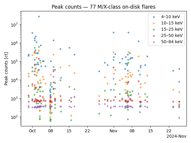
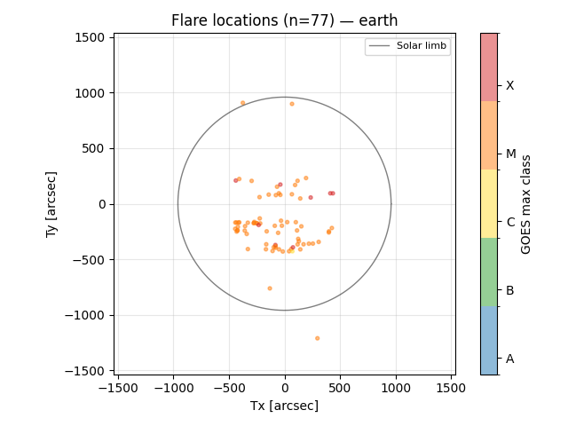
Selected 77 M/X-class on-disk flares of 7025 total.
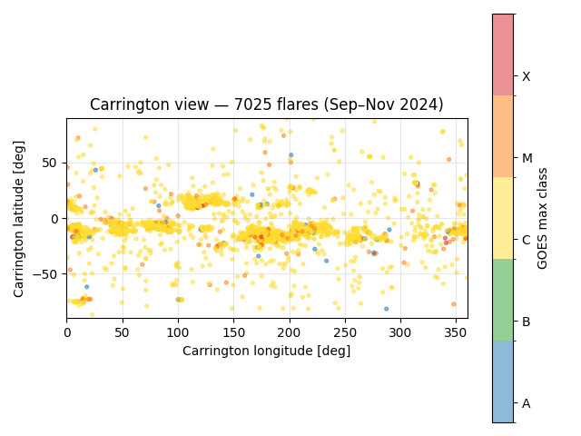
Plotting a catalogue that spans many weeks onto a single Earth-view Sun disc is misleading: solar rotation moves features ~13°/day, so a persistent active region smears into a horizontal streak across the disc and individual flares are no longer comparable in position.
A rotation-fixed view solves this. observer="carrington" plots
heliographic Carrington longitude (0–360°) vs latitude — the Carrington
prime meridian rotates with the Sun, so an active region keeps the same
longitude across many days. Each flare’s own Solar Orbiter position is used
as the HGC observer, matching how STIX actually saw the event.
flares.plot_locations(observer="carrington")
plt.title(f"Carrington view — {len(flares)} flares (Sep–Nov 2024)")
plt.tight_layout()
plt.show()
Total running time of the script: (3 minutes 40.258 seconds)